MRtrix3教程 #6 Connectome
简介
现在我们已经创建了一个流线图,我们就可以创建一个连接组,代表连接大脑不同部分的流线数量。为了做到这一点,我们必须首先将大脑分割成不同的区域,或节点。做到这一点的一个方法是是使用脑图谱(atlas),将大脑中的每个体素分配给特定的ROI。
你可以使用你想要的任何脑图谱,但在本教程中,我们将使用FreeSurfer附带的脑图谱。因此,我们的第一步将是通过recon-all来处理被试的解剖图像。
# 如果想更换数据生成的目录,可以设置SUBJECTS_DIR环境变量到自己想要的目录路径
$ export SUBJECTS_DIR=<your_custom_path>
# 耗时很长,需要慢慢等。
$ recon-all -i sub-CON02_ses-preop_T1w.nii.gz -s sub-CON02_recon -all
创建脑连接组(Connectome)
当recon-al完成后,我们将需要把FreeSurfer解析的标签转换为MRtrix能理解的格式。labelconvert命令将使用FreeSurfer的注解(parcellation)和分割输出来创建一个新的.mif格式的注解(parcellation)文件:
$ labelconvert -help
MRtrix 3.0.4                      labelconvert                       Dec 14 2022

     labelconvert: part of the MRtrix3 package

SYNOPSIS

     Convert a connectome node image from one lookup table to another

USAGE

     labelconvert [ options ] path_in lut_in lut_out image_out

        path_in      the input image

        lut_in       the connectome lookup table corresponding to the input
                     image

        lut_out      the target connectome lookup table for the output image

        image_out    the output image
$ labelconvert sub-CON02_recon/mri/aparc+aseg.mgz $FREESURFER_HOME/FreeSurferColorLUT.txt /usr/local/mrtrix3/share/mrtrix3/labelconvert/fs_default.txt sub-CON02_parcels.mif
然后,我们需要创建一个全脑连接组,代表图谱中每个注解对之间的流线(本例中为84x84)。“symmetric” 选项将使下对角线与上对角线相同,而 “scale_invnodevol"选项将以节点大小的倒数来缩放连接组:
$ tck2connectome -h
MRtrix 3.0.4                     tck2connectome                      Dec 14 2022

     tck2connectome: part of the MRtrix3 package

SYNOPSIS

     Generate a connectome matrix from a streamlines file and a node
     parcellation image

USAGE

     tck2connectome [ options ] tracks_in nodes_in connectome_out

        tracks_in    the input track file

        nodes_in     the input node parcellation image

        connectome_out  the output .csv file containing edge weights
...
Options for outputting connectome matrices

  -symmetric
     Make matrices symmetric on output

  -zero_diagonal
     Set matrix diagonal to zero on output
     ...
  -out_assignments path
     output the node assignments of each streamline to a file; this can be used
     subsequently e.g. by the command connectome2tck
     ...


$ tck2connectome -symmetric -zero_diagonal -scale_invnodevol -tck_weights_in sift_1M.txt tracks_10M.tck sub-CON02_parcels.mif sub-CON02_parcels.csv -out_assignment assignments_sub-CON02_parcels.csv
可视化脑连接组
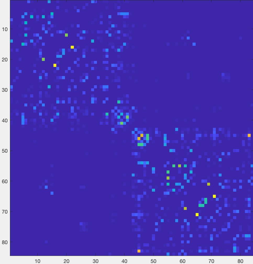
创建parcels.csv文件后,我们可以在Matlab中将其视为矩阵。首先,需要导入它:
connectome = importdata('sub-CON02_parcels.csv')
% 更高的结构连接对更亮
imagesc(connectome)
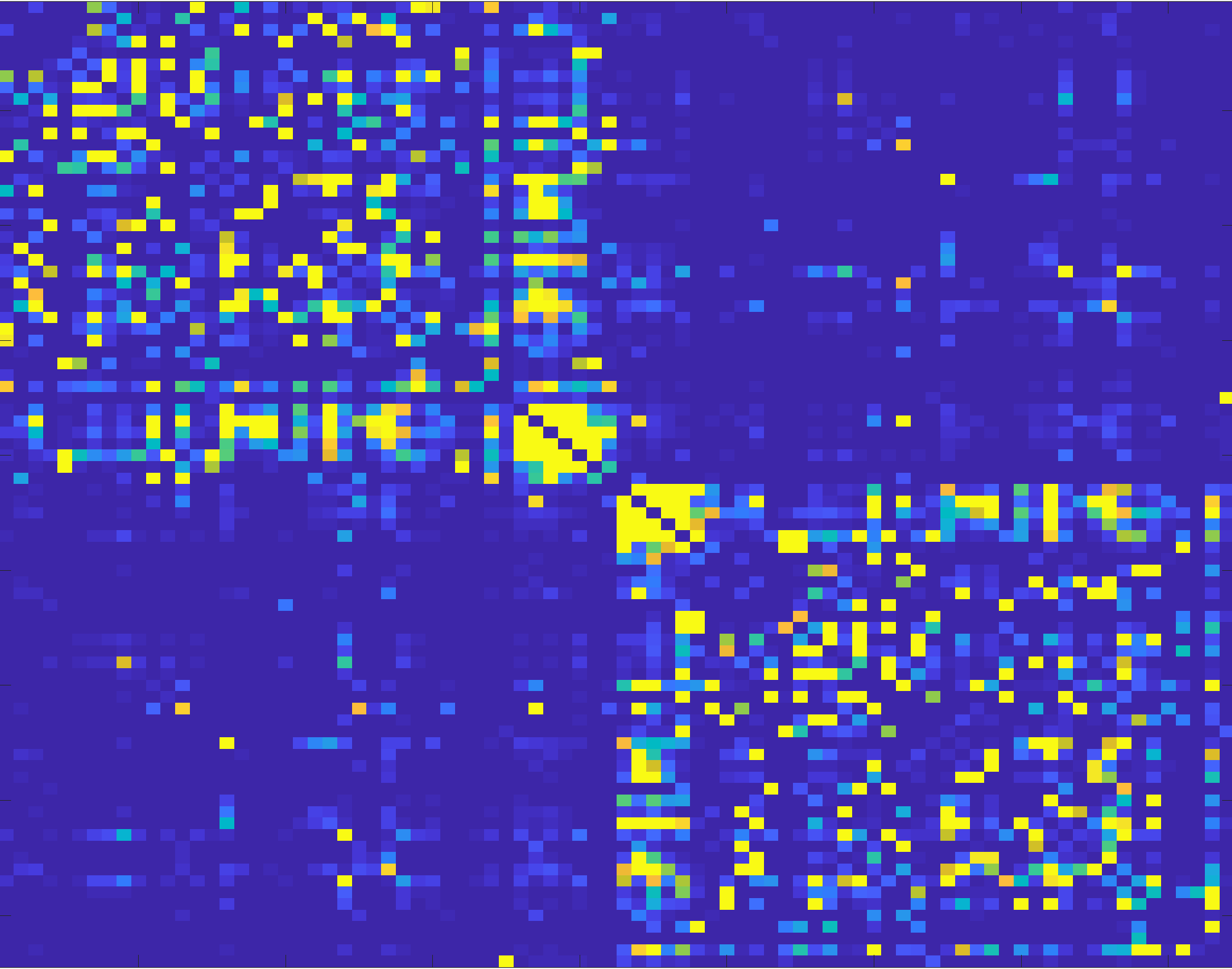
% 为了使这些关联更加明显,您可以更改颜色图的缩放比例
imagesc(connectome,[0,1])